I was reading this interesting preprint on ordinal regression by Paul Bürkner and Matt Vuorre. Now see this footnote about their vocabulary:

Hallelujah and Eureka!! I think that these terms may help solve (some of) the long-standing confusion about the difference between “fixed” and “random” effects.

TL;DR: To shrink or not to shrink – that is the question

The mathematical distinction is that Varying (“random”) parameters have an associated variance while Population-level (“fixed”) parameters do not. Population-level effects model a single mean in the population. Varying effects model a mean and a variance term in the population, i.e., two rather than one parameters. The major practical implication is that Varying parameters have shrinkage in a regression towards the mean-like way whereas the Population-level parameters do not.

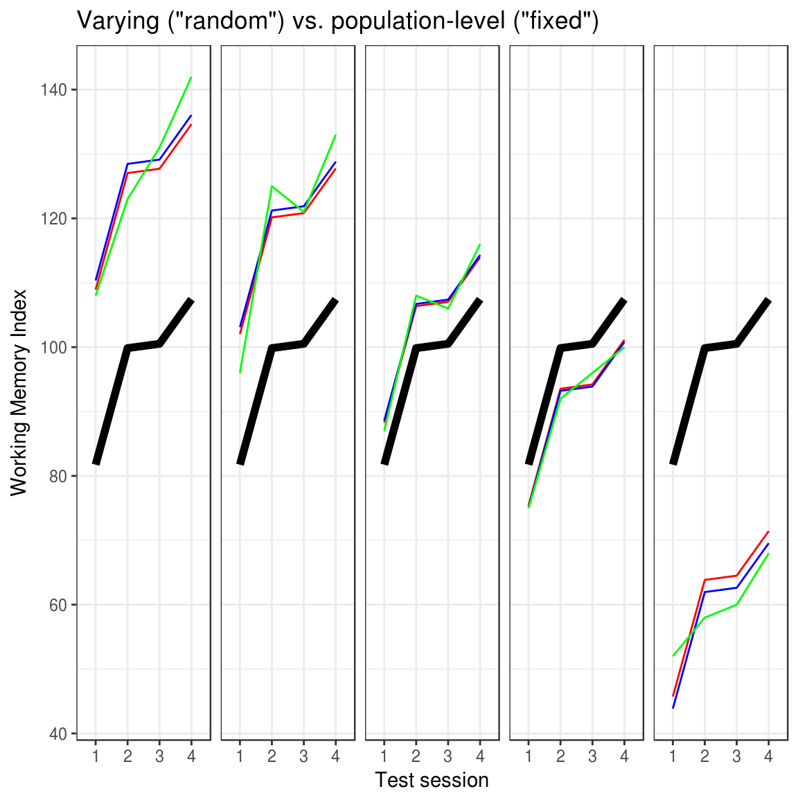
The figure below shows this shrinkage in action for the following three models:

fit_varying = lme4::lmer(WMI ~ session + (1|id), D)  # Varying subject-intercept (red lines)
fit_population = lm(WMI ~ session + id, D)  # Population-level subject-intercept (blue lines)
fit_mean = lm(WMI ~ session, D)  # No subject-intercept (black lines)

The figure shows five illustrative participants (panels), each tested four times. A model with varying subject-intercept (red lines) shrinks subjects closer to the group mean (black line) than the model with the population-level subject-intercept (blue lines). The green lines are actual scores. Furthermore, the shrinkage is stronger the further away the data is from the overall mean. See the accompanying R notebook for all details and all participants.

So shrinkage is the only practical difference. This is true for both frequentist and Bayesian inference. Understanding when to model real-world phenomena using shrinkage, however, is not self-evident. So let me try to unpack why I think that the terms “Population-Level” and “Varying” convey this understanding pretty well.

Population-level parameters

General definition:

Values of Population-level parameters are modeled as identical for all units.

Example:

Everybody in the population of individuals who could ever be treated with X would get an underlying improvement of exactly 4.2 points more than had they been in the control group. Mark my words: Every. Single. Individual! The fact that observed changes deviate from this true underlying effect is due to other sources of noise not accounted for by the model.

The example above could be a 2×2 RM-ANOVA model of RCT data (outcome ~ treatment * time + (1|id)) with treatment-specific improvement (the treatment:time interaction) as the population-level parameter of interest. Populations could be all people in the history of the universe, all stocks in the history of the German stock market, etc. Again, the estimated parameters are modeled as if they were exactly the same for everyone. The only thing separating you from seeing that all-present value is a single residual term of the model, reflecting unaccounted-for noise. The residual is an error term so it is not the model itself. As seen from the model, everybody is identical and the residual is simply an error term (which is not part of the model) indicating how far this view of the world deviates from observations.

I think that modeling anything as a Population-level parameter is an incredibly bold generalization of the sort that we hope to discover using the scientific method: the simplest model with the greatest predictive accuracy.

Now, it’s easy to see why this would be called “fixed” when you have a good understanding of what it is, but as a newcomer,  the term “fixed” may lead you astray thinking that either (1) it is not estimated, (2) that it is fixed to something, or that its semantically self-contradictory to call a variable fixed! Andrew Gellman calls them non-varying parameters, and I think this term suffers a bit from the same possible confusions. Population-level goes a long way here. The only ambiguity left is whether parameters that apply to the population also apply to individuals, but I can’t think of a better term. “Universal”, “Global”, or “Omnipresent” are close competitors but they seem to generalize beyond a specific population so let’s stick with Population-level.

Varying parameters

General definition:

Values of Varying parameters are modeled as drawn from a distribution.

Example for (1|id) :

Patient-specific baseline scores vary with SD = 14.7.

Example for (0 + treatment:time | id) :

The patient-specific responses to the treatment effect vary with SD = 3.2 points.

This requires a bit of background explaining so bear with me: Most statistics assume that the residuals are independent. Independence is a fancy way of saying that if you know any one residual point, you would not be able to guess above chance about any other residuals. Thus, the independence assumption is violated if you have multiple measurements from the same unit, e.g., multiple outcomes from each participant since knowing one residual from an extraordinary well-performing participant would lead you to predict above-chance that other residuals from that participants would also be positive.

You could attempt to solve this by modeling a Population-level intercept for each participant (outcome ~ treatment * time + id), effectively subtracting that source of dependence in the model’s overall residual. However, which of these participant-specific means would you apply to an out-of-sample participant? Answer: none of them; you are stuck (or fixed?). Varying parameters to the rescue! Dropping the ambition to say that all units (people) exhibit the same effect, you could estimate the recipe on how to generate those intercepts for each participant which helped you get rid of the dependence of the residuals (or more precisely: model it as a covariance matrix). This is a generative model in the form of the parameter(s) of a distribution and in GLM this would be the standard deviation of a normal distribution with mean zero.

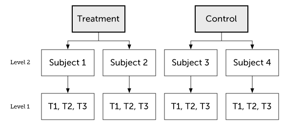
One way to represent this clustering of variation to units is a hierarchical model where outcomes are sampled from individuals which are themselves sampled from the nested Population-level parameter structure:

For this reason, I think that we could also call Varying parameters sampled parameters. This is true whether those sampled parameters are intercepts, slopes, or interaction terms. Crossed Varying effects are just parameters sampled from the joint distribution of two non-nested populations (e.g., subject and questionnaire item). Simple as that!

Again, it’s easy to see why one would call this a “random” effect. However, as with “fixed effects,” it is just easy to confuse this for (1) the random-residual term in the whole model, or (2) the totally unrelated difference between frequentist and Bayesian inference as to whether data or parameters are fixed or random. Varying seems to capture the what it’s all about – that units can vary in a way that we can model. With variation comes regression towards the mean so it follows naturally.

Two derived properties of Varying

Firstly, it models regression towards the mean for the varying parameters: Extreme units are shrunk towards the mean of the varying parameter since those units are unlikely to reflect a true underlying value. For example, if you observe an exceptionally large treatment effect for a particular participant, he or she is likely to have experienced a lesser underlying improvement, but unaccounted-for factors exaggerated this by chance. Similarly, when you observe exceptionally small observed treatment effects, it is likely to reflect a larger underlying effect masked by chance noise.

Secondly, it requires enough levels (“samples”) of the Varying factor to estimate its variance. You just can’t make a very relevant estimate of variance using two or three levels (e.g. ethnicity). Similarly, sex would definitely make no sense as Varying since there is basically just two levels. Participant number, institution, or vendor would be good for analyses where there are many different of those. For frequentist models like lme4::lmer, a rule of thumb is more than 5-6 levels. For Bayesian models, you could have even one level (because Bayes rocks!) but the influence of the prior and the width of the posterior would be (unforgivably?) big.

Some potential misunderstandings

I hope that I conveyed the impression that the distinction between Population-level and Varying modeling is actually quite simple. However, the Fixed/Random confusion has caused people to exaggerate their difference for illustrative purposes, giving the impression that they do have distinct “magical properties”. I think they are more similar:

Both random and fixed can de-correlate residuals: It is sometimes said that you model effects as “fixed” to model effects of theoretical interest and other effects as “random” to account for correlated residuals, thus respecting the independence assumption (e.g., repeated measures). However, both “fixed” and “random” effects de-correlate residuals with respect to that effect. No magic!

Both random and fixed can account for nuisance effects: It is often said that random effects are for nuisance effects and fixed effects model effects of theoretical importance. However, as with the point above about de-correlating residuals, they can both do this. Say you want to model some time-effect (e.g., due to practice or fatigue) of repeated testing to get rid of this potential systematic disturbance if your theory-heavy parameters. You could model time as a fixed effect and just ignore its estimate or you could model it as random. The decision should not be theory vs. nuisance but rather whether the effect of time is modeled as identical for everyone or as Varying between units. No magic!

Both Varying and Population-level are model population-wide parameters. The word “population-level” effect may sound like it is the only parameter that says something about the population or that it is easier to generalize. In fact, I highlighted above that for “sampled” parameters, it was easier to see how Varying effects would generalize. Is this self-contradictory? No. Population-level effects are the postulate that there is a single mean in the population. Varying effects are the postulate that there is a mean and a variance term in the population.

Helpful sources

A few sources that helped me arrive at this understanding was:

1. Here are some nice visualizations of “fixed” vs. “random” effects in the context of meta-analyses. The distinction is the same. Instead of “study”, just think “participant”, “country”, or whatever.
2. Writing mixed models in BUGS helped me to de-mysticise most of linear models, including fixed/random and what interactions are. I started in JAGS. Here’s a nice example.
3. This answer on Cross-Validated which made me realize that shrinkage is the only practical difference between modeling parameters as “fixed” or “random.”
4. The explanation in the FAQ to R mailing list on GLMM, primarily written by the developers of the lme4 package.
5. Brauer & Curtin (2017) with plain-language recommendations for mixed models.
6. Hodges & Clayton (2011) makes a distinction between “old-style” random effects (draws from a population), which I have mentioned here, and “new-style” random effects where the variance term is used more for mathematical convenience, e.g. when there is no population, the observed units exhaust the population, or when no new draws are possible. It is my impression that “new-style” is seldom used in psychology and human clinical trials.

TO DO

• IMPORTANT: Rename terms? Varying is just two population-level parameters instead of one. How about: “
• Mention that population-level has superior fit to data.
• Fix plot annotations
• Varying as uncertainty around fixed and residual as errors from model!
• Use intro model in the quotes below
• Fixed vs. random well-known in MA
• Add legend to figure