$$\sqrt{2}$$ is superior to Bessel’s correction

… for the estimation of the population standard deviation. That is, if you substitute $$n – 1$$ with $$n – \sqrt{2}$$, you get a much less biased estimate of the population SD. I just stumbled upon this when I desperately (!) looked to frequentist methods because of convergence problems with my bayesian model. The details can be seen in my post on Cross Validated about this curious finding as well as some excellent answers/elaborations.

I’m re-posting the simulation results here, just because they’re pretty and I want some content on this blog.

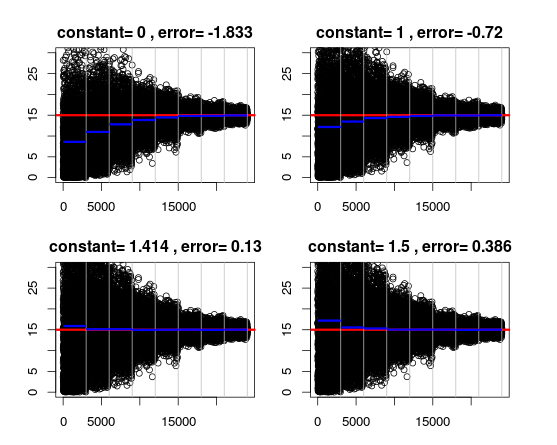
TL: no correction. TR: Bessel’s correction. BL: $$\sqrt{2}$$ correction (superior). BR: 1.5. Red: real population sd. Blue: estimated sd (corrected). Gray lines indicate different sample size with 3000 simulations per sample size. Click on the image to view the script.

Naturally, $$\sqrt{2}$$ doesn’t outperform the analytically correct solution but it is a surprisingly good approximation. For larger sample sizes (n > 10), $$n – 1.5$$ becomes superior. In any case, it’s a nice reminder that Bessel’s correction does NOT magically make the sample SD into a population SD as is currently taught in many statistics classes.

I’m considering adding this fun-fact to the Wikipedia page on unbiased estimation of the standard deviation, where you can read more about the issue of bias in frequentist estimation.

.

This PNAS paper could be the go-to example of how not to interpret statistics

A few days ago, a science reporter asked me to evaluate a PNAS paper titled Gender differences in the structural connectome of the human brain. As it turns out, this paper is awful. On the positive side, it’s an excellent opportunity to highlight common mistakes in psychology/neuroscience and how to do it (more) properly.

1. Minute effect sizes do not allow for bold generalizations

From abstract:

In all supratentorial regions, males had greater within-hemispheric connectivity, as well as enhanced modularity and transitivity, whereas between-hemispheric connectivity and cross-module participation predominates in females.

The paper generalizes it’s significant findings of structural brain differences between males and females to ALL males and females. Let’s evaluate how wrong you’d be to take the author’s conclusion for granted (using Common Language effect size): If you guess that a randomly picked female has got more between-hemispheric connections than a randomly picked male, you’d be wrong more than 41 % of the time. And for their second major conclusion: If you do the same tests, guessing male superiority with respect to within-hemispheric connections, you’d be wrong at least 37 % of the time. It is outright frightening to think of the possibility that policy makers could be influenced by this paper!

2. Don’t do reverse inference when you can do forward inference

From abstract:

“Overall, the results suggest that male brains are structured to facilitate connectivity between perception and coordinated action, whereas female brains are designed to facilitate communication between analytical and intuitive processing modes”.

The authors say that the (minute) structural differences explain behavioral differences between genders. This is reverse inference which can be very uninformative when applied to macrostructures such as lobes or hemispheres (read: small effect size). Therefore the same critique applies as above.

It is particularly strange that the authors did collect gender-relevant behavioral data on all subjects (see page 4, right column) but they do not statistically test them against the structural connectivity of said subjects. This is more than obvious to do if they wanted to claim that the structural differences underlie behavioral gender differences, and it could shut down critics like me if it showed a convincing relationship. The fact that they didn’t explicitly test to what extent the relationship between individual’s connectivity and behavior is modulated by gender makes me worry that it does not.

3. Interaction is required to claim developmental differences

From abstract:

“Analysis of these changes developmentally demonstrated differences in trajectory between males and females, mainly in adolescence and adulthood”.

… but the age x sex interaction is non-significant (page 3, right column). Thus it is invalid to conclude that sexes develop differently as a major part of this difference might be present at the outset. This is an all too common error in neuroscience.

4. Keep conclusions close to what’s actually tested

From abstract:

between-hemispheric connectivity and cross-module participation predominates in females.

and from significance-section:

”female brains are optimized for interhemispheric connections.

… yet they only statistical test it on connections between frontal lobes. It’s a quite violent generalization to equate a frontal lobe with a hemisphere. Figure 2 clearly indicates that almost only connections between frontal lobes are significant in females. E.g. there are no parietal-parietal or temporal-frontal connections. It seems very post-hoc (only report significant findings), and it’s certainly not a valid generalization.

Conclusion

If we remove the invalid parts of the abstract (and the study motivation), here’s what’s left:

“In this work, we modeled the structural connectome using diffusion tensor imaging in a sample of 949 youths (aged 8–22 y, 428 males and 521 females). Connection-wise statistical analysis, as well as analysis of regional and global network measures, presented a comprehensive description of network characteristics.”

… which is just a description of what they did without any interpretations. This is exactly the part that I like about the paper. The design is good, the data set is very impressive, and the modeling of connections between regions seems valid. I’d love to see these data in the hands of other researchers.

The fact that this paper got published in its current form is frankly discouraging for PNAS, for peer-review and the reputation of neuroscience. Let’s hope that cases like this only generalizes to the same extent as the conclusions of this paper do.

.

Renaming Brain Vision Recorder EEG recordings

Renaiming Brain Vision Recorder files is a pain. Here’s a python script that makes it (more of) a breeze.

The problem

Brain Vision Recorder is a widely used software for EEG-recordings. Every EEG-recording is saved as three files:

  1. One .eeg file, containing all the data
  2. One .vmrk/.amrk/.bmrk file, containing markers and a reference to the .eeg file
  3. One .vhdr/.ahdr/.bhdr file, containing header information and references to the marker file and data file. This is the file that represents the recording and opened by analysis software

Because of these internal references between the files, it is quite laborious (and risky) to rename a recording. I often rename my recordings before analysis. I use the Python script below for this purpose.

The script

import os, fileinput

# Specify folder with .eeg and meta-files
folder = '/home/jonas/Desktop/test/'

# Loop through all files
for filename in sorted(os.listdir(folder)):
    filebase, filetype = os.path.splitext(filename)

    # Only operate on selected file extensions
    if filetype in ('.eeg', '.bhdr', '.vhdr','.ahdr','.bmrk','.amrk','.vmrk'):
        print 'processing '+filename+'...'

        # Generate new name
        newname = 'XXXX' + filename

        # Actually rename file
        os.rename(folder+filename,folder+newname)

        # Updates header and marker files to match actual filenames
        filebase, filetype = os.path.splitext(newname)
        if filetype != '.eeg':
            for line in fileinput.FileInput(folder +newname, inplace=1):
                # For header-files and marker-files
                if 'DataFile=' in line: line = 'DataFile='+filebase+'.eeg'

                # For header-files
                elif 'MarkerFile=' in line:
                    tmp_str = 'MarkerFile='+filebase
                    if filetype == '.bhdr': tmp_str +='.bmrk'
                    if filetype == '.ahdr': tmp_str +='.amrk'
                    if filetype == '.vhdr': tmp_str +='.vmrk'
                    line = tmp_str
                print line.replace('\n','')

How to modify the script

The important part is just below the “#Generate new name”. You can use this in two ways. First, you can rename your files in the browser and type in

newname = filename

This will simply update the header information in the header- and marker-files. Secondly, you can use all sorts of generative filename generation. E.g. this takes a subject ID from the middle of the filename and adds it to the front after a paradigm-name:

newname = 'aud-oddball, subject ' +filename[6:10] + filename[:6] + filename[10:]

I hope this helps someone out there.

Calculating d’, beta, c and Ad’ in Python and PHP

About d’

A central component of Signal Detection Theory is d’ – a measure of the ability to discriminate a signal from noise. The d’ is flanked by the parameters “beta” and c, which are measures of the criterion that the observer uses to discriminate between the two.

These measures can be calculated in every experiment where there is a signal (e.g. target trials) and noise (e.g. nontarget trials), and the observer (e.g. subject) is to indicate whether the signal was present or not. d’, beta and c are statistical measures in a model where noise and noise+signal are regarded as two “probability-of-detection” distributions on a “threshold-of-detection” continuum. d’ is basically a Z-score on how well the observer discriminates the two distributions, i.e. the number of standard deviations between the probability-of-response distributions for signal and noise for this given subject. c (the criterion) is the number of standard deviations from the midpoint between these two distributions, i.e. a measure on a continuum from “conservative” to “liberal”.

Every trial is scored as one of four possibilities:

  • noise + signal + response: HIT
  • noise + signal + no response: MISS
  • noise + response: FALSE ALARM (FA)
  • noise + no response: CORRECT REJECTION (CR)

It is often analyzed in terms of rates:

  • HIT RATE = HIT/SIGNALS (ratio of signals detected as signals)
  • FA RATE = FA/NON-SIGNALS (ratio of noise detected as signals)

You want to have a high hit rate and a low fa rate (hitrate > farate). Say you have conducted an experiment on a subject and calculated hitrate and farate. A signal-detection account of the subjects signal-detection-abilities can be one of the following

  • If hitrate=1 and farate=0, d’ is infinite, meaning that you signals and noise are totally separated, i.e. the distributions are non-overlapping. In that case, you have effectively discriminated signal from noise.
  • If hitrate > farate, d’ is positive, meaning that you are more likely to detect the information as signal when signal is present than when it is absent.
  • If hitrate=farate, d’=0, meaning that you are just as likely to detect signals and noise as signals, i.e. you were unable to discriminate the signal and noise and hence the probability-of-detection distributions overlap perfectly. This occurs when responses are perfectly random.
  • If hitrate < farate, d’ is negative, meaning that you have a wierd bias of primarily detecting noise as signals while ignoring the actual signals.
  • If hitrate = 0 and farate = 1, d’ is negatively infinite, meaning that you have completely confused noise and signal.

For a a more thorough introduction and guide to calculating d’/beta, “Calculation of signal detection theory measures” by Stanislaw & Todorov.

Calculating d’, beta, c and Ad’ in Python

Using the Percentile Point Function (ppf) from scipy:

from scipy.stats import norm
import math
Z = norm.ppf

def SDT(hits, misses, fas, crs):
    """ returns a dict with d-prime measures given hits, misses, false alarms, and correct rejections"""
    # Floors an ceilings are replaced by half hits and half FA's
    half_hit = 0.5 / (hits + misses)
    half_fa = 0.5 / (fas + crs)
 
    # Calculate hit_rate and avoid d' infinity
    hit_rate = hits / (hits + misses)
    if hit_rate == 1: 
        hit_rate = 1 - half_hit
    if hit_rate == 0: 
        hit_rate = half_hit
 
    # Calculate false alarm rate and avoid d' infinity
    fa_rate = fas / (fas + crs)
    if fa_rate == 1: 
        fa_rate = 1 - half_fa
    if fa_rate == 0: 
        fa_rate = half_fa
 
    # Return d', beta, c and Ad'
    out = {}
    out['d'] = Z(hit_rate) - Z(fa_rate)
    out['beta'] = math.exp((Z(fa_rate)**2 - Z(hit_rate)**2) / 2)
    out['c'] = -(Z(hit_rate) + Z(fa_rate)) / 2
    out['Ad'] = norm.cdf(out['d'] / math.sqrt(2))
    
    return(out)

Note the adjustment of rate=0 and rate=1, to prevent infinite values.

Calculating d’, beta, c and Ad’ in PHP

// Percentile Point Function from http://spechal.com/2009/11/15/php-function-to-emulate-excel-normsinv/
function Z($p){
	$a1 = -39.6968302866538; $a2 = 220.946098424521; $a3 = -275.928510446969;
	$a4 = 138.357751867269; $a5 = -30.6647980661472; $a6 = 2.50662827745924;
	$b1 = -54.4760987982241; $b2 = 161.585836858041; $b3 = -155.698979859887;
	$b4 = 66.8013118877197; $b5 = -13.2806815528857; $c1 = -7.78489400243029E-03;
	$c2 = -0.322396458041136; $c3 = -2.40075827716184; $c4 = -2.54973253934373;
	$c5 = 4.37466414146497; $c6 = 2.93816398269878; $d1 = 7.78469570904146E-03;
	$d2 = 0.32246712907004; $d3 = 2.445134137143; $d4 = 3.75440866190742;
	$p_low = 0.02425; $p_high = 1 - $p_low;
	$q = 0.0; $r = 0.0;
	if($p < 0 || $p > 1) throw new Exception("NormSInv: Argument out of range.");
	else if($p < $p_low){
		$q = pow(-2 * log($p), 2);
		$ppf = ((((($c1 * $q + $c2) * $q + $c3) * $q + $c4) * $q + $c5) * $q + $c6) / (((($d1 * $q + $d2) * $q + $d3) * $q + $d4) * $q + 1);
	} 
	else if($p <= $p_high){
		$q = $p - 0.5; $r = $q * $q;
		$ppf = ((((($a1 * $r + $a2) * $r + $a3) * $r + $a4) * $r + $a5) * $r + $a6) * $q / ((((($b1 * $r + $b2) * $r + $b3) * $r + $b4) * $r + $b5) * $r + 1);
	} 
	else {
		$q = pow(-2 * log(1 - $p), 2);
		$ppf = -((((($c1 * $q + $c2) * $q + $c3) * $q + $c4) * $q + $c5) * $q + $c6) / (((($d1 * $q + $d2) * $q + $d3) * $q + $d4) * $q + 1);
	}
	return $ppf;
}
 
// Credit to comment on http://php.net/manual/en/function.stats-stat-percentile.php
function erf($x) { 
        $pi = 3.1415927; 
        $a = (8*($pi - 3))/(3*$pi*(4 - $pi)); 
        $x2 = $x * $x; 
 
        $ax2 = $a * $x2; 
        $num = (4/$pi) + $ax2; 
        $denom = 1 + $ax2; 
 
        $inner = (-$x2)*$num/$denom; 
        $erf2 = 1 - exp($inner); 
 
        return sqrt($erf2); 
}
 
function cdf($n) { 
        if($n < 0) return (1 - erf($n / sqrt(2)))/2; 
        else return (1 + erf($n / sqrt(2)))/2; 
}
 
// Calculate d' and avoid infinity
function dPrime($hits, $misses, $fas, $crs) {
	$half_miss = 0.5/($hits+$misses);
	$half_fa = 0.5/($fas+$crs);
	$hitrate = $hits/($hits+$misses);
	$farate = $fas/($fas+$crs);
 
	// Avoid d' negative infinity
	if($hitrate < 0.025) {
		if($hitrate+$half_miss < 0.025) $hitrate = 0.025;
		else $hitrate = $half_miss;
	}
	if($farate < 0.025) {
		if($farate+$half_fa < 0.025) $farate = 0.025;
		else $farate = $half_fa;
	}	
 
	// Avoid d' infinity
	if($hitrate > 0.975) {
		if($hitrate-$half_miss > 0.975) $hitrate = 0.975;
		else $hitrate = 1-$half_miss;
	}
	if($farate > 0.975) {
		if($farate-$half_fa > 0.975) $farate = 0.975;
		else $farate = 1-$half_fa;
	}
 
	// Calculate d' using Percentile Point function
	$out = new stdClass;
	$out->d = Z($hitrate)-Z($farate);
	$out->beta = exp((pow(Z($farate),2) - pow(Z($hitrate),2))/2);
	$out->c = -(Z($hitrate)+Z($farate))/2;
	$out->Ad = cdf($out->d/sqrt(2));
	return $out;
}

Note that a rate-threshold of 0.025 is used because the PHP-ppf function above is only an estimation which fails violently if this threshold is exceeded.

The case for PsychoPy

Most researchers in cognitive neuroscience have to program an experiment in a stimulus-delivery environment at some time in their career. Everyone have heard about Presentation and E-prime but much fewer have heard about PsychoPy – a free cross-platform stimulus delivery environment.

PsychoPy logo

Advantages over Presentation and E-Prime:

  1. Free and open source, meaning no license problems!
  2. Cross-platform. You can develop on Windows, Mac or Linux and run your experiment on Windows, Mac and Linux!
  3. Limitless functionality. Psychopy is a Python module, which means that it can be heavily extended with other Python modules for e.g. Matlab-level matrix operations (numpy), image and audio manipulations, advanced statistics etc.
  4. Flexible stimulus-handling: “Online” stimulus-generation, e.g. random-noise masks or moving Gaussian gratings. Also, you can define stimuli-sizes in degrees relative to the subject’s eyes, rather than having to do the trigonometry yourself.

Timing:

It compares to E-Prime and Presentation on timing. I’ve tested it on our stimulus-facilities using a photosensitive diode and comparing the timing of stimuli-appearance on the monitor to the triggers sent on a parallel port. It is reliably below 0,1 ms.

In PsychoPy you can (optionally) define durations of stimuli in monitor-frames rather than milliseconds, which ensures that timing is very well-controlled.

Disadvantages:

  1. PsychoPy’s timing of audio stimuli is still not perfect. I’ve found a ~10ms jitter in audio onset (I’ve seen much worse in some C-compiled experiments…). If you need very precise audio timing, go for something else.
  2. The serious experimenter still needs to script all of his experiment. Although a very nice graphical interface is in development, it is still not thoroughly tested and tried. In my oppinion programming in Python is much cleaner and easier than E-Prime and Presentation.

Getting started:

Good introduction to Python syntax: Learn Python in 10 minutes
Download PsychoPy at PsychoPy.org and read documentation here.

Computing half-area latency in matlab/EEGLAB

In EEG research the latency of a component (hidden in the ERP) is conventionally measured as the time when the ERP is most extreme. However, this method is not well warranted, as should be clear to anyone who have read Steven Lucks excellent chapters on ERP analysis in “An Introduction to the Event Related Potential Technique”. Instead he proposes a 50% area latency method: the latency is the point in time where the area under the curve is equal on both sides. It yields the same latencies as peak-measures on symmetrical ERPs and more correct latencies on non-symmetrical ERPs, where peak-measures fails.

A first solution

If you have your ERP as an array in MATLAB, you can compute the 50% area in this way:

erp = [1,2,3,4,5,6,7,8,9,7,4,2,-2,3]; #ERP data, one point for each sample.
[~,latency_index] = min(abs(cumsum(erp)-sum(erp)/2)); #Index in array that best divides it into 50-percent area

To use it with EEGLAB (assuming you have your epoched EEG structure) you might implement it in this way:

#Get the ERP waveform as erp_data. Insert the channel-number, e.g. 5 for Fz.
[~,~,~,~,~,erp] = pop_erpimage(EEG,1, channel, [], [], 1, 1, {}, [], '', 'erp','on','noshow','on');

#Only use the part of the ERP that represents the component you're analyzing, e.g.
samples = 100:200;
erp = erp(samples);

#Get the index in the ERP, as above.
[~,latency_index] = min(abs(cumsum(erp)-sum(erp)/2))

#Get the index in milliseconds from stimulus onset.
latency_ms = (EEG.xmin + (samples(1)+latency_index)/EEG.srate)*1000;

How it works

Let’s have a look at how this works. Remember that we want to find the sample where the area is equal on both sides. It consists of the following steps:

  1. Transform the erp array into an array of cumulative sums, i.e. every element is the sum of all previous elements. E.g. the array erp=[1,3,4,0] becomes erp_cumsum = [1,4,8,8]. (try to imagine this ERP to ease your understanding). Each element then corresponds to the area that precede it in the ERP. The last element corresponds the total area of the ERP.
  2. Now the job is simply to find the midmost value in erp_cumsum, i.e. the value that separates the area into two equal parts. To do this, we subtract the half area from every element in erp_cumsum. Continuing the example from above, sum(erp)/2 = 4. The subtraction giveserp_reduced = erp_cumsum-sum(erp)/2 = [-3,0,5,5].
  3. The midmost value in erp_cumsum is now the element closest to zero (we can already see that this is sample number 2). Finding it in matlab is done by taking the absolute value, which gives erp_abs = abs(erp_reduced) = [3,0,5,5], and finding the index of the minimum value. This is simply [~,index] = min(erp_abs).

Correction: defining the direction of the component

This method is not fool-proof but things can be done to prevent some errors. Consider a positive ERP (e.g. P300) that starts and ends at negative values, .e.g erp = [-3,0,5,2,-1,-4]. This is a very nice peak and visually you would consider it all to be part of the P300. However, using cumulative sums, the start and end would be “negative area”, which doesn’t make sense when we’re trying to find a latency.

The solution starts off by defining whether you’re looking for the latency of a positive or a negative peak. Then you adjust your ERP to only contain positive or negative values by raising or lowering the whole ERP so that all elements have the same sign. In this example, we’re looking for a positive component and then we raise the ERP by 4. If we were looking for a negative component, we’d lower the ERP by 5. So:

# For positive components:
erp_adjusted = erp-min(erp) = [1,4,9,6,3,0]; 

# For negative components:
erp_adjusted = erp-max(erp) = [-8,-5,-3,0,-6,-9];

Extending it to multiple ERPs

Say you’re dealing with multiple ERPs and want to calculate 50% latencies on all of them. You want to put in e.g. 50 ERPs and get 50 latencies as output. This is practical if you want to calculate latencies on individual trials to investigate variability or on multiple subjects at the same time. This is where Matlab’s excellent matrix operations get to work. I don’t want to go into details on this one. I’m just going to give you the code for positive-going components in single-trial ERPs:

samples = 100:200;
erp_matrix = pop_erpimage(EEG,1, channel, [], [], 1, 1, {}, [], '','noshow','on');
erp_adjusted = bsxfun(@minus,erp_matrix(samples,:),min(erp_matrix(samples,:)));
[~,latency_indicies] = min(abs(bsxfun(@minus,cumsum(erp_adjusted),sum(erp_adjusted)/2)));
latencies = (EEG.xmin + (samples(1)+latency_indicies)/EEG.srate)*1000;